Markov Chains

Markov chains is an interesting concept with applications in several disciplines. Markov chains are stochastic processes with a specific property called Markov property. This post presents the definitions of stochastic processes and Markov chains with examples. It describes the Markov property and various related characteristics of Markov chains like transition distribution, stationary distribution, absorbing states and absorbing Markov chains.

Stochastic process

A stochastic process describes a random phenomenon over time. Random variables are used to model the random phenomenon of a stochastic process, thus, a stochastic process is a sequence of random variables indexed by time. Since these random variables model the same phenomenon, i.e., the state of the phenomenon, therefore, they share the domain (i.e., the state space) and the range. The time index could be discrete or continuous, resulting in discrete-time or continuous-time stochastic processes respectively.

An example of a stochastic process could be as simple as flipping of an unbiased coin at every second for a minute. We can model it as a sequence of sixty independent and identically distributed (iid) random variables based on Bernoulli distribution with its parameter as 0.5. A complex example could be some noise in an electric circuit over time, stock market over time or Brownian motion.

Formally, a stochastic process is a sequence of random variables $X_1$, $X_2$, … $X_t$ representing the states at time $1, 2, …, t$. Further, the initial probability distribution $Pr(X_1)$ and the probability distributions of the subsequent states should be specified. The distribution of the state at at time $t+1$ is described as a conditional distribution conditioned on the observed states {$X_1 = x_1$, $X_2 = x_2$, …, $X_t = x_t$}. The joint distribution of the sequence can be written as:

\[Pr(X_1=x_1,X_1=x_2, ..., X_t=x_t) = \\ Pr(X_1=x_1) Pr(X_2=x_2|X_1=x_1) ... \\ Pr(X_t=x_t|X_{1}=x_{1}, X_{2}=x_{2}, ..., X_{t-1}=x_{t-1})\]

Markov chains

A Markov chain is a special kind of stochastic process, which obeys the Markov property. The Markov property states that the conditional probability distribution of the next state depends only on the current state. This property is also called memorylessness, in contrast with a general stochastic process, it does not matter what the past states are, only the current state decides the next state. Mathematically, the property is stated as:

\[Pr(X_{t+1}=x|X_1=x_1,X_1=x_2, ..., X_t=x_t) = Pr(X_{t+1}=x|X_t=x_t)\]

Using this property, we can write the joint distribution of the sequence as:

\[Pr(X_1=x_1,X_1=x_2, ..., X_t=x_t) = \\ Pr(X_1=x_1) Pr(X_2=x_2|X_1=x_1) ... Pr(X_t=x_t|X_{t-1}=x_{t-1})\]

Note: One might say that $X_3$ does depend on $X_1$ because $X_2$ depends on $X_1$, and it is indeed correct. $X_3$ does depend on $X_1$. However, the assumption is that $X_3$ depends only on $X_2$. That is, given $X_2$, $X_3$ does not depend on $X_1$. Another way to understand the Markov property is that $X_3$ is independent of $X_1$ given $X_2$, that is: $P(X_3 | X_2, X_1) = P(X_3 | X_2)$.

To summarize, Markov property states that the next state does not depend on the past given the present.

Examples

The game of snakes and ladder is an example of Markov chains. A player can be in one of the hundred states corresponding to the hundred positions on the board. The next position, i.e., state is decided by the current state and the roll of the dice. Note that the next state is decided by the current state alone, it does not matter how the current state is attained.

Flipping an unbiased coin sixty times for a minute is also an example of a Markov chain. This is called a Bernoulli process, the underlying probability distribution is a Bernoulli distribution with the parameter 0.5. This is an extremely simple case, where the next state is not even dependent on the current state.

The state space of a Markov chain could be continuous as well. Consider an example with the conditional probability distribution at $t+1$ as: $Pr(X_{t+1} | X_t = x_t) = N(x_t, 1)$. Here the state space is real numbers, and the next state is specified as a normal distribution with its mean as the current state and variance 1.

Following is another example of a Markov chain. We have a grid of 3 elements, numbered 1, 2 and 3. The rules of the movement are that the position can only change horizontally, and the position has to be in the grid. The probability of moving left or right is 0.5 each. In case of the first and the last position, the probability of moving right and left is 0.5 respectively, and probability to stay in the position is 0.5 for both the positions. The state transition diagram shows the probabilities on the edges of the possible transitions.

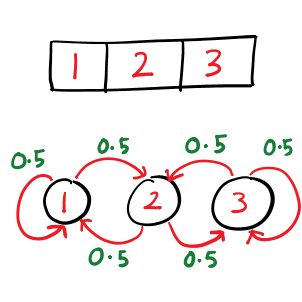
The conditional distribution for this Markov chain is the following: $p_{11} = 0.5$, $p_{12} = 0.5$, $p_{13} = 0$, $p_{21} = 0.5$, $p_{22} = 0$, $p_{23} = 0.5$, $p_{31} = 0$, $p_{32} = 0.5$, $p_{33} = 0.5$.

Transition distribution

For a given set of states ($S$), we can write the conditional probability distribution at time $t+1$ as $Pr(X_{t+1}=j|X_t=i)$ for the states $i, j \in S$. This conditional distribution is called transition distribution, representing the probability of state change from $i$ to $j$ at time $t+1$. The transition distribution is stationary if it remains the same for all values of $t$. We can write the stationary transition distribution from state $i$ to $j$ as $Pr(X_{t+1}=j|X_t=i) = p_{ij}$ for all values of $t$.

Matrix form of transition distribution (transition matrix) for the grid example:

\[P = \begin{bmatrix} p_{11} & p_{12} & p_{13} \\ p_{21} & p_{22} & p_{23} \\ p_{31} & p_{32} & p_{33} \end{bmatrix} = \begin{bmatrix} 0.5 & 0.5 & 0 \\ 0.5 & 0 & 0.5 \\ 0 & 0.5 & 0.5 \end{bmatrix}\]

Multi-step transition matrix

If P is the transition matrix of a Markov chain, i.e., transition distribution of a single step then, $P^m$ will give the transition matrix of $m$ steps. In other words, $P^m$ represents probability of going from one state to another in exactly $m$ steps.

Stationary distributions

At any point of time, the process could possibly in any one of the $k = |S|$ states with some probability. We can define a probability vector or probability distribution representing the probability of being in each state. Let it be a matrix $\nu$ of dimension $1 X k$. Further, we can represent the probability vector at time $t+1$ in terms of probability vector at $t$ and transition matrix:

\[\nu_{t+1} = \nu_t P\]

Stationary distribution are those probability vectors ($\nu_s$) that remains the same after multiplication with the transition distribution. Another name of stationary distribution is equilibrium distribution, i.e., Markov chain is in an equilibrium.

\[\nu_s P = \nu_s\]

Note that the equation looks similar to the one of eigenvalues and eigenvectors. Precisely, $\nu_s$, i.e., stationary distribution of a Markov chain is a left eigenvector of the transition matrix.

Theorem: If there exists a value of $m$ such that $P^m$ has all values greater than zero then:

• The Markov chain has a unique stationary distribution $\nu_s$
• All the rows of the matrix $\lim_{n \rightarrow \infty} P^n$ would be $\nu_s$, that is:

\[\begin{bmatrix} \nu_s \\ \nu_s \\ \vdots \\ \nu_s \end{bmatrix} = \lim_{n \rightarrow \infty} P^n\]

Absorbing Markov chains

A state $i$ of a Markov chain is called an absorbing state if $p_{ii} = 1$, i.e., once the state is attained, the state never changes. In other words, the state keeps changing to itself.

A Markov chain is called absorbing Markov chain if an absorbing state can be reached, in one or more steps, from all the states of the Markov chain.