Neural Network Backpropagation

The learning process in machine learning involve determining the weights of a model that minimize a loss function. Usually, gradient based techniques are used to learn the weights. Gradient based techniques rely on the computation of gradients of the loss function w.r.t. the weights. Backpropagation is a widely used algorithm to efficiently compute these gradients.

Backpropagation at a high level is simply a recursive application of the chain rule of calculus while avoiding repetitive computations. Specifically, it is a dynamic programming based solution for computing the gradients involving the chain rule of calculus.

This post presents the mathematical formulation of backpropagation for neural networks. It presents the notation of neural networks, the forward equations and the backpropagation equations.

Notation

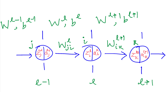
• $u^l$: number of units in layer $l$
• $W^l_{ji}$: weight between layer $l-1$ and $l$ from unit $i$ to unit $j$ respectively
• $W^l$: weight matrix between layers $l-1$ and $l$ of dimension ($u^{l-1}, u^l$)
• $b^l$: bias vector at layer $l$ of dimension ($u^l$)
• $g^l$: activation function at layer $l$
• $a^l_{i}$: activation of unit $i$ of layer $l$
• $a^l$: activations of layer $l$ of dimension ($u^l, 1$)
• $z^l_{i}$: input to activation function of unit $i$ of layer $l$
• $z^l$: input to activation function of layer $l$ of dimension ($u^l, 1$)

Forward propagation

For each layer $l+1$, we compute $z^{l+1}$ and $a^{l+1}$ using the following forward equations. In each step, $a^l$ of the previous layer is used to compute the $a^{l+1}$ of the current layer. For the base case, i.e., for the first layer, $a^l$ of the previous is the input of the network. The output of the network is the $a$ values computed in the last layer.

• $z_{i}^{l+1} = \sum_{j=1}^{u^l} W^{l+1}_{ji} a^l_j + b^{l+1}_i$
• $a^{l+1}_i = g^{l+1}(z^{l+1}_i)$

The same equations in matrix form:

• $z^{l+1} = (W^{l+1})^T a^l + b^{l+1}$
• $a^{l+1} = g^{l+1}(z^{l+1})$

Backward propagation

The goal of backpropagation is to compute the derivatives of loss function w.r.t. weights at every layer for a given dataset. That is, given a dataset $(X, Y)$, we want to compute $\frac{\partial L}{\partial W_{ji}^l}$ and $\frac{\partial L}{\partial b_i^l}$ for all values of $i$, $j$, and $l$.

The output of a network is a function of the weights and the input (X). Further, the loss of a network is a function of its output and the expected output (Y). Note that the variables X and Y are constants in the loss function. Thus, loss function is effectively a function of the weights of the network once the values of (X, Y) are supplied.

We compute the derivatives by applying the chain of differentiation several times. Specifically, the derivatives at layer $l$ are dependent on the derivatives of the layer $l$. Thus, the derivatives computation flows backward hence the name backpropagation.

For each layer, we compute $\delta_j^l = \frac{\partial L}{\partial z_j^l}$. The computation of $\delta_j^l$ is done recursively in terms of $\delta_i^{l+1}$. Once we have $\delta_j^l$, we can compute $\frac{\partial L}{\partial W_{ij}^l}$ and $\frac{\partial L}{\partial b_j^l}$ in terms of the same.

The loss function is a function of the output of the network, however, the output can written in terms of the $z^l$ at every layer. As a result, we can write loss completely in terms of $z^l$ for every layer. Formally, we can express $\delta_i^l$ as follows:

$\delta_j^l = \frac{\partial L(z^{l+1})}{\partial z_j^l}$ = $\frac{\partial a_j^l}{\partial z_j^l}\frac{\partial L(z^{l+1})}{\partial a_j^l}$ = $\frac{\partial g^l(z_j^l)}{\partial z_j^l} \frac{\partial L(z^{l+1})}{\partial a_j^l}$

Using the chain rule of calculus for mutiple variables, we write:

$\delta_j^l = \frac{\partial g^l(z_j^l)}{\partial z_j^l} \sum \limits_{i=1}^{u_{l+1}} \frac{\partial L(z^{l+1})}{\partial z^{l+1}_i} \frac{\partial z^{l+1}_i}{\partial a_j^l}$

$\delta_j^l = \frac{\partial g^l(z_j^l)}{\partial z_j^l} \sum \limits_{i=1}^{u_{l+1}} \delta_i^{l+1} W_{ji}^{l+1}$

In matrix form the equation can written as:

$\delta^l = \frac{\partial g^l(z_j^l)}{\partial z_j^l} \odot (W^{l+1} * \delta^{l+1})$

where $\odot$ is element wise product, i.e., Hadamard product.

Base case: when $l$ is the last layer, $\delta_i^l$ can be computed directly. There is no need of recursion, simple differentiation can be used.

Gradients w.r.t. parameters

$\frac{\partial L}{\partial W_{ji}^l} = \frac{\partial z_i^l}{\partial W_{ji}^l} \frac{\partial L}{\partial z_i^l}$ = $a_j^{l-1} \delta_i^l$

$\frac{\partial L}{\partial b_i^l} = \frac{\partial z_i^l}{\partial b_i^l} \frac{\partial L}{\partial z_i^l}$ = $1 * \delta_i^l$ = $\delta_i^l$

Note that the mechanism avoids re-computations of the gradients of the later layers. This makes the backpropagation algorithm efficient.

Example

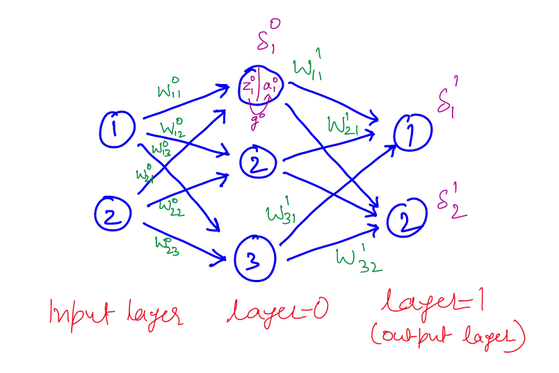
For this examples the forward equations for first unit of layer 0 are:

• $z_{1}^{0} = W_{11}^0 x_1+ W_{21}^0 x_2$
• $a^{0}_0 = g^{0}(z^{0}_0)$

The backprop equations for computing $\delta_1^0$ are:

• $\frac{\partial L}{\partial a_1^0} = \delta_1^{1} W_{11}^{1} + \delta_2^{1} W_{12}^{1}$ : backprop from $\delta^1$ to $a_1^0$
• $\delta_1^0 = \frac{\partial g^0(z_1^0)}{\partial z_1^0} (\delta_1^{1} W_{11}^{1} + \delta_2^{1} W_{12}^{1})$ : backprop from $a_1^0$ to $z_1^0$

The equations for computing derivatives w.r.t. weights are:

$\frac{\partial L}{\partial W_{11}^1} = \frac{\partial z_1^1}{\partial W_{11}^1} \frac{\partial L}{\partial z_1^1}$ = $a_1^{0} \delta_1^1$

$\frac{\partial L}{\partial b_1^1} = \frac{\partial z_1^1}{\partial b_1^1} \frac{\partial L}{\partial z_1^1}$ = $1 * \delta_1^1$ = $\delta_1^1$

Appendix: Chain Rule of Calculus (Multivariate)

$L$ is a function of $a$ and $b$, which are function of $x$. The derivative of $L$ w.r.t. $x$ can be computed as follows:

$\frac{d L(a, b)}{d x} = \frac{\partial L(a, b)}{\partial a} \frac{da}{dx} + \frac{\partial L(a, b)}{\partial b} \frac{db}{dx}$