Manjeet Dahiya
Gradient Descent
Gradient descent is one of the most popularly used optimization technique for learning models like linear regression, logistic regression and deep learning. All the major machine learning frameworks, namely TensorFlow, Sci-kit learn and Keras, provide multiple solvers (a.k.a, optimizers), and most of which are just different variations of gradient descent.
Goal of these ML frameworks is to minimize a loss function (also called cost function) for a given training dataset. The optimization algorithm enables these frameworks to find the parameters of the model such that the loss function is minimum.
It is very important to build an understanding of gradient descent so that one can choose the variant of gradient descent wisely as well as debug the same during the training phase. This will allow the user to comprehend the results and determine if the algorithm has really converged to the minima.
This post presents the details of gradient descent and hope to build insights on how this algorithm works. An implementation of the same is also provided with examples. Finally, it presents the advantages and disadvantages of gradient descent.
Concept
First and foremost, gradient descent is simply an optimization technique. That is, given a functions $f(x)$, its goal is to determine the value of $x$ such that $f(x)$ is minimum.
Machine learning is just another field where gradient descent finds its application. It turns out that gradient descent and its variants are quite suitable to the need of machine learning. Other than this, gradient descent is an independent concept altogether having its roots in the field of mathematical optimization.
Gradient descent is an iterative procedure that keeps getting closer to the minima in each step, and finally, converges to the minima modulo the given tolerance error. It is a first-order numerical method as the computation uses the first derivative of the given function.
We pick a random value of the candidate minima and keep changing it until the convergence. In each step of gradient descent, the current value of the candidate minimum is moved in the direction opposite to the gradient. That is, in each step, $x$ is set to $x - \eta f’(x)$, where $f’(x)$ is the derivative (i.e., gradient) of $f(x)$ and $\eta$ is some positive value. Note that the gradient gives the direction of the steepest ascent, i.e., the direction for $x$ that would increase the value of $f(x)$ the most. Since our objective is to find the minima, we greedily take the opposite direction (i.e., $-f’(x)$) resulting in the steepest descent of $f(x)$. We keep taking these steps until the gradient converges to zero. Note that the gradient is zero at the minima point for convex functions.
For convex functions, the above mentioned steps will keep moving the candidate minima to the actual minima. For examples, $f(x) = x^2$ is minimum at $x=0$ and its gradient is $f’(x) = 2x$. For points $x < 0$ and $\eta = 0.1$, the gradient will be negative, consequently, the value of $x$ will move to the right. On the other hand, for $x > 0$, the gradient is positive and the algorithm will shift it to the left. The algorithm will converge when the value of gradient is very small, i.e., $x$ is in the neighborhood of zero.
More on gradient
This section explains more about gradient, especially, in higher dimensions. The gradient of a function $f(x, y)$ is defined as:
\[\nabla f = \frac{\partial f(x, y)}{\partial x} \hat{\mathbf{x}} + \frac{\partial f(x, y)}{\partial y} \hat{\mathbf{y}}\]It is a vector, $\hat{\mathbf{x}}$ and $\hat{\mathbf{y}}$ represent unit vector in the direction of $x$ and $y$ axis respectively. The value of vector in each direction is the partial derivative of $f$ w.r.t. the variable corresponding to the axis. $\nabla f$ represent the direction where the value of $f$ will increase the most, and its magnitude represents the magnitude of the increase in the value of $f$.
We can now write the gradient descent equation for its iterative step. Given a multi-dimensional function $f(X)$ as the function of input vector X. Here the number of dimensions of $f$ is $len(X)$. The change performed in $X$ in each step is:
\[X = X - \eta \nabla f\]Where $\eta$ is some positive number, also called the learning rate or step size.
Formulation and implementation
Following the the three important components of any iterative numerical method. initialization, iteration step and convergence, i.e., termination. In gradient descent initialization is starting with a random value of the candidate minima. The iteration step is $x = x - \eta f’(x)$ and the solution is said to converged if $abs(f’(x)) < threshold$, i.e., the magnitude of the gradient is below some given small threshold.
The function $gradient\_descent$ of the following Python program implements gradient descent for functions with single variable. It takes three arguments:
- $grad$: a callable representing the gradient of the target function
- $threshold$: the precision in the minima achieved. Smaller value for $threshold$ will result in better approximation of the minima.
- $step\_size$ is a positive value representing $\eta$ in our formulation.
Finally, it computes and prints the minima of the function $f(x) = x^2 + x$. Note that the function $grad\_fx$ returns the gradient of $x^2 + x$.
import random

def gradient_descent(grad, threshold=0.001, step_size=0.1):
    x = random.random()                     # initialization
    while not (abs(grad(x)) < threshold):   # convergence check
        x = x - step_size * grad(x)         # iteration step
    return x

def grad_fx(x):
    # returns the gradient of fx = x^2 + x
    return 2 * x + 1

print(gradient_descent(grad_fx))
# prints -0.499
It is straightforward to extend this implementation for multi-dimensional functions.
Significance of the step size (learning rate)
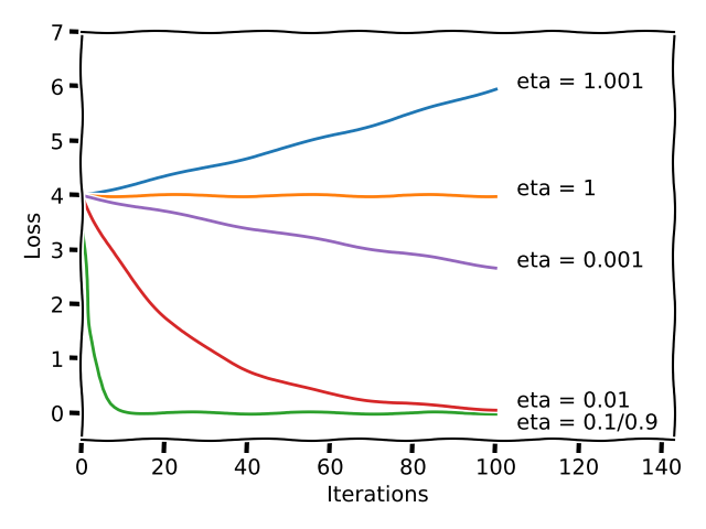
The step size is a hyperparameter of gradient descent. Its value can have significant impact on the convergence of gradient descent. The diagram below shows the effect of different values of $\eta$ for $f(x) = x^2$. The loss (i.e., $x^2$) is plotted with iteration count for each value of $\eta$.
- $\eta = 0.1, 0.9$: Convergence is fast.
- $\eta = 0.01$: Convergence is slow.
- $\eta = 0.001$: Convergence is extremely slow.
- $\eta = 1$: Loss is constant, the value of $x$ keeps oscillating between 2 and -2.
- $\eta = 1.001$: Loss keeps increasing and diverges.
A good idea is to try multiple values of $\eta$, e.g., 0.5, 0.1, 0.01 and 0.01 and analyze the loss values with iterations. Thus, one can figure out if the optimizer is converging at a reasonable speed.
Another issue one must be aware of that the value of $eta$ is same for all the dimensions. This can lead to a problem if the different inputs are not scaled to a same range. We may not be even able to find a suitable $\eta$ that can lead to convergence. A good idea to deal with this issue is to scale all the different inputs to a same range.
Limitations
Gradient descent is computationally suitable for machine learning optimization goals. For example, the closed form solution of linear regression requires matrix inversion of size $D X D$ where $D$ is the number of features/dimensions. The complexity of this solution is $O(D^3)$, which is huge. In practice, gradient descent converges much faster. Moreover, its variants like stochastic gradient descent (SGD) are quite suitable for machine learning, where the data could be huge and SGD allows to work with the batches of the data.
However, gradient descent comes with problems of its own:
- For non-convex functions gradient descent doesn’t guarantee a the global minimum. Depending upon the initialization and the value of $\eta$ it is quite possible that it results in an unwanted local minimum, saddle point or inflection point.
- Gradient descent requires the first derivative of the given function. What if the first derivative does not exit for the objective function?
- Step size tuning is a problem. Ideally, we do not want to worry about oscillations, divergence and slow convergence. There are variants of gradient descent that help resolve this issue. I will cover those in the future posts.
© 2018-19 Manjeet Dahiya