Markov Chains Modeling for Gambler's Ruin Problem

This post presents an application of Markov chains and related ideas. This post models the Gambler’s Ruin Problem as a Markov chain, and presents its solution.

Gambler’s Ruin Problem

There are many variations of the problem with the same essence. Here is another.

Two players A and B play a game with the following rules:

• A fair coin is tossed. Player A wins on heads, and Player B wins on tails.
• The player that loses transfers one unit of money to the winner, and then the game is continued, and the coin is tossed again.
• The game terminates when one of the players is ruined, i.e., has zero money left to play with.

The money they start with is $R_A$ and $R_B$ respectively. We need to find the probability of winning of a player.

Markov chain modeling

Let us simplify the problem by setting small, concrete values of $R_A$ and $R_B$ to 1 and 2 respectively. At each step of the game, $R_A$ can increment or decrement by one, with equal probabilities. Since the total money in game is 3, there are four possibilities for $R_A$ in the game: \(\{0, 1, 2, 3\}\). The game ends when $R_A$ is either 0 (A loses all the money) or 3 (B loses all the money). The game continues for the other two states.

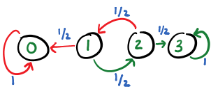
Let us denote this game as a state transition diagram. A state represents the current amount of money A has, and an edge represents a transition between states. Note that the state of player A alone is sufficient to capture the state of the game, as the total money in the game is constant, i.e, $R_A + R_B = 3$. The following figure shows the state transition diagram. A node denotes the money that player A has, i.e., $R_A$. When the game is in state 2, player A can lose to go to state 1 or she may win to go to state 3. The probability in states 1 and 2 for winning and losing the current step is determined by tossing a fair coin and is 0.5 each. The states 0 and 3 indicate termination of the game. Once these states are attained there is no way going to another state.

The game follows the Markov property. The conditional probability of the next move is independent of the previous states. Moreover, the Markov chain described by the transitions is an absorbing Markov chain. States 0 and 3 are absorbing states, and these absorbing states can be reached by all the other states in one or more steps. This implies that the game will reach a steady state.

The transition distribution for the game is the following:

\[P = \begin{bmatrix} p_{00} & p_{01} & p_{02} & p_{03} \\ p_{10} & p_{11} & p_{12} & p_{13} \\ p_{20} & p_{21} & p_{22} & p_{23} \\ p_{30} & p_{31} & p_{32} & p_{33} \end{bmatrix} = \begin{bmatrix} 1 & 0 & 0 & 0 \\ 0.5 & 0 & 0.5 & 0 \\ 0 & 0.5 & 0 & 0.5 \\ 0 & 0 & 0 & 1 \end{bmatrix}\]

Computing limiting probability distribution

Let $\nu$ denote the probability distribution of states, i.e., probability of the game being in any particular state. It is a 1x4 matrix, representing the probability of each state. If $\nu_t$ is the probability distribution of states at time $t$, then $\nu_{t+1}$ can be computed by the following equation:

\[\nu_{t+1} = \nu_t P\]

We are given that the initial value of $P_A$ is 1, therefore, the initial probability distribution is

\[\nu_0 = [0, 1, 0, 0]\]

We can compute the probability distribution after one step, two steps, three steps, ten steps and hundred steps as follows:

\[\nu_{1} = \nu_0 P = [0.5, 0, 0.5, 0]\] \[\nu_{2} = \nu_0 P^2 = [0.5, 0.25, 0, 0.25]\] \[\nu_{3} = \nu_0 P^3 = [0.625, 0, 0.125, 0.25]\] \[\nu_{10} = \nu_0 P^{10} = [0.66601562, 0.00097656, 0, 0.33300781]\] \[\nu_{100} = \nu_0 P^{100} = [\approx 0.6666, \approx 0, \approx 0, \approx 0.3333]\]

$\nu_{100}$ denotes that after 100 steps the probability that the game is in losing state (state 0) is 2/3, and the game is in winning state (state 3) is 1/3. Moreover, the probability that game is still not terminated is almost zero, i.e., the probability being in states 1 and 2.

Interpreting the result

A game between A and B, with starting money 1 and 2 respectively, has 1/3 probability such that A wins. On the other hand, player B, who starts with more money, has 2/3 (higher) probability of winning. For a general case, we can prove that the probability that A wins is $R_A/(R_A+R_B)$. In other words, it is better to start with more money than the opponent. Note that the general can can be solved by a similar argument. It would require constructing a transition matrix of size $(R_A+R_B+1) X (R_A+R_B+1)$, and then computing the limiting distribution.

Conclusion

Markov chains can be used to solve the problems that obey the Markov property. One has to just model the problem as a Markov chain and the rest comes for free. One can then reason in terms the existing results on Markov chains.